Frequency Response of Second-Order Systems

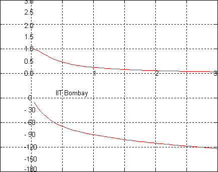
The animated plot below shows the magnitude and phase of the transfer function ${\frac {1}{s^2 + 2{\zeta}{{\omeag}_n} + {{\omega}_n}^2}}$ plotted as a function of the non-dimensional ratio ${\Omega}={\frac {\omega}{{\omega}_n}}$ of the input frequency $\omega$ to the natural frequency $\omega_{\rm n}$ for different values of the damping ratio ${\zeta}$. The magnitude and phase of the transfer function at the frequency $\omega$ gives the amplification and phase shift that a sinusoidal input of frequency $\omega$ undergoes as it passes through the system.   In the magnitude plot, the non-dimensional frequency ratio ${\Omega}$ takes values in the range 0 to 3 while the damping ratio ${\zeta}$ decreases from  2 to 0. The plots corresponding to the values $2$, ${\sqrt 2}$, 1, ${\frac {1}{\sqrt 2}}$ and ${\frac {1}{2{\sqrt 2}}}$ for the damping ratio ${\zeta}$ are shown in red. The plot for ${\zeta}=0$ shows the frequency response of an undamped system, while  ${\zeta}=1$ corresponds to a critically damped  system. The values ${\zeta}={\sqrt 2}, 2$ correspond to an overdamped system, while ${\zeta}={\frac {1}{\sqrt 2}}$, ${\frac {1}{2{\sqrt 2}}}$ correspond to an underdamped system. 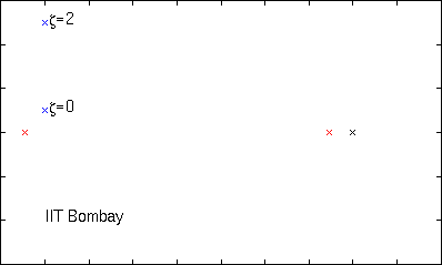The value${\zeta}={\frac {1}{\sqrt 2}}$ is the smallest value of damping ratio for which the system shows no amplification at any input frequency. The animated plot on the right shows the movement of the poles of the system as the damping ratio ${\zeta}$ varies.

Notice that as the damping ratio ${\zeta}$ approaches 0 the magnitude increases at every frequency. The magnitude at ${\Omega}=1$ increases to ${\infty}$ as ${\zeta}$ approaches 0. This phenomenon is known as resonance. At resonance, the phase equals $90^{\circ}$ for all values of ${\zeta}$. Also, as ${\zeta}$ increases  to ${\frac {1}{\sqrt{2}}}$, the input frequency corresponding to the maximum amplification shifts lower away from resonance ( ${\Omega}=1$).

The same information is also shown on the animated plot below using a log scale for the frequency, which varies in the range $10^{-2} {\rm rad/s}  {\rm to}  10^2 {\rm rad/s}$. The magnitude is plotted in decibels  (1 decibel  =  20 log  (magnitude)),  while the phase is plotted in degrees on a linear scale. Frequency response information plotted in this fashion is referred to as a Bode plot. 

                                                           The animation appearing on this page was created with help from Debashish Bagg.